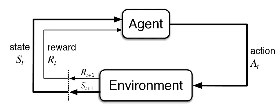
I was studying reinforcement learning a while ago, attempting to educate myself about deep Q learning. As part of that effort, I read through the first few chapters of Reinforcement Learning: An A Introduction by Sutton and Barto. Here are my notes on Chapter 3. Like all of my other notes, these were never intended to be shared, so apologies in advance if they make no sense to anyone.

Chapter 3

Agent-Environment Interface

They mainly cover basic terminology here. The main difference from bandit problems is that the state can change with each action.

• $\mathcal{S}$ = state space, $\mathcal{A}$ = action space, $\mathcal{R}$ = reward space. These are all finite, with $\mathcal{R} \subseteq \mathbb{R}$.

• As with the bandit problems, we have $A_t$, $R_t$ are the actions and rewards at time $t$. The book uses $R_{t+1}$ to denote the reward given for action $A_t$. MDPs introduce another time series, $S_t$ to denote the state at time $t$. Thus $S_t$ and $A_t$ "go together" and $S_{t+1}$ and $R_{t+1}$ are "jointly determined."

• The probability distributions governing the dynamics of an MDP are given by the density function:

  $$p(s', r\,\vert\, s,a) := \mathbb{P}(S_{t+1} = s', R_{t+1} = r\,\vert\,S_t=s,A_t=a)$$

  Other useful equations are:

  $$p(s'\,\vert\,s,a) = \sum_{r\in\mathcal{R}}p(s',r\,\vert\,s,a), \\ r(s,a) := \mathbb{E}[R_t\,\vert\,S_{t-1}=s,A_{t-1}=a] = \sum_{r\in\mathcal{R}}\sum_{s\in\mathcal{S}}p(s',r\,\vert\,s,a) \\ r(s,a,s') := \mathbb{E}[R_t\,\vert\,S_{t-1}=s,A_{t-1}=a,S_t=s'] = \sum_{r\in\mathcal{R}}r\cdot\frac{p(s',r\vert s,a)}{p(s'\vert s,a)}$$

Goals and Rewards

Note that as with bandit problems, $R_t$ is stochastic. But this is also the only thing we can really tune about a given system. In pactice, reward is based on the full state-action-state transition, and therefore the randomness comes from the environment.

Key insight: keep rewards simple with small, finite support. For some reason, I think of this as an extension of defining really simple prior distributions. Since in this case, the value (return) is determined by percolating rewards backwards from terminal states.

Returns and Episodes

Define a new random variable $G_t$ to be the return at time $t$. So if an agent interacts for $T$ time steps, this would be defined

Unified Notation for Episodic and Continuing Tasks

Here, the book allows $T$ to be infinite. In this ncase, we need a discounting factor for future returns, or otherwise the return would be a potentially divergent series. Let $\gamma$ be the discount factor (possibly equal to 1 for finite episodes), so that

This unified notation is defined after discussing terminal states, which help to deal with the problem of finite episodes. A terminal state is a sink in the state-action graph, whose reward is always zero. This allows us to always use infinite sums even for finite episodes.

Policies and Value Functions

A policy is a conditional distribution over actions, conditioned on a state:

The value of a state is the expected return, with respect to the policy distribution:

The quality of an action $a$ at state $s$ is the expected return

We call $q_\pi$ the action-value function.

Exercise 3.12

Give an equation for $v_\pi$ in terms of $q_\pi$ and $\pi$.

Solution:

Exercise 3.13

Give an equation for $q_\pi$ in terms of $v_\pi$ and the four-argument $p$.

Solution:

The fourth line follows from the third because of the Markov property.