Notes on Reinforcement Learning 2

January 28, 2023

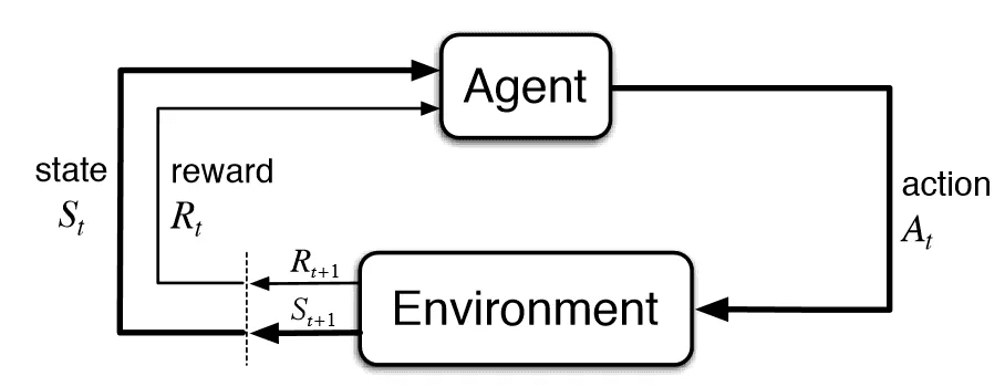
I was studying reinforcement learning a while ago, attempting to educate myself about deep Q learning. As part of that effort, I read through the first few chapters of Reinforcement Learning: An A Introduction by Sutton and Barto. Here are my notes on Chapter 2. Like all of my other notes, these were never intended to be shared, so apologies in advance if they make no sense to anyone.

Chapter 2

The simplest RL problems are those that omit or fix one aspect of the dynamics. In the Stanford lectures, we started with Markov Reward Processes, which are MDPs without actions. In Sutton and Barto, we first study multiarmed bandit problems, which are MDPs with a single state.

Bandit Problems

Since we have only one state, there is no real distinction between reward and value. We therefore talk of the optimal value function as the expected reward:

q_\ast(a) = \mathbb{E}(R_t | A_t = a).

To contrast with general MDPs, the value function would be the expected discounted sum of future rewards. But this is consistent with the above equation, since we have

\begin{aligned} q_\ast(a) &= \mathbb{E}\bigg[\sum_{i=0}^\infty R_{t+i}\gamma^i \bigg\vert A_t = a\bigg] \\ &= \mathbb{E}(R_t\vert A_t=a) + \gamma\cdot\mathbb{E}\bigg[\sum_{i=0}^\infty R_{t+i+1}\gamma^i \bigg\vert A_t = a\bigg] \\ &= \mathbb{E}(R_t\vert A_t=a) + \gamma\cdot\mathbb{E}\bigg[\sum_{i=0}^\infty R_{t+i+1}\gamma^i \bigg], \end{aligned}

where the final step follows because $R_i$ is independent of $A_t$ for $i>t$ . Therefore, the expectation of future rewards is constant with respect to $t$ , and so we can set the discount factor $\gamma = 0$ . This is a form of an identity that shows up a lot in the study of MDPs, called the Bellman equation.

Note that actions and rewards are random variables. This is to allow us to model complex systems as stochastic if there are two many factors to allow for a deterministic model. This will be the case for all RL systems that I read about in this book. The goal for multiarmed bandit problems will be to estimate $q_\ast$ , because once the value function is known, the optimal strategy is to pick the action which maximizes $q_\ast$ . In the next sections, we will define an estimator $Q_t(a)$ for $q_\ast(a)$ that we update as we play. Using stochastic policies that allow us to explore, we can iteratively improve the estimator and hope for convergence.

Action-Value Methods

The most obvious estimator for $q_\ast$ is the historical average of rewards when action $a$ was taken:

Q_t(a) = \frac{\sum_{i=0}^{t-1}R_i\cdot\mathbb{1}_{A_i=a}}{\mathbb{1}_{A_i=a}}.

Using this value function, we can define various policies:

Greedy - Define $A_t = \text{argmax}_aA_t(a).$
$\epsilon$ -greedy_ - For fixed $\epsilon\in(0,1)$ , let $A_t = \text{argmax}_aA_t(a).$ with probability $1-\epsilon$ and let $A_t$ be chosen uniformly from the remaining actions with total probability $\epsilon$ .

Those are defined in the book. Another one that comes to mind is to select actions according to the distribution $\mathbb{P}(a) = \text{softmax}(Q_t(a))$ .

Incremental Implementation

The book motivates this section by talking about how calculation of sample averages grows linearly in complexity, and therefore they need to be cached and updated iteratively. This is true, but it feels like a way out of explaining Markov properties and Bellman equations until later. Fix an action $a$ and redefine $R_i$ to denote the reward received the $i$ th time the action $a$ was taken. Then if $a$ was chosen $n$ times, define

Q_{n+1} = \frac{1}{n}\sum_{i=1}^nR_i.

Then note that $Q_{n+1} = Q_n + \frac{1}{n}[R_n Q_n]$ (this calculation is carried out in the book). This has the form

\text{newEstimate} = \text{oldEstimate} + \text{stepSize}\cdot\text{error},

which will show up often in the book.

Nonstationary Bandit Problems

We say a bandit problem is nonstationary if the reward distributions depend on $t$ . In this event, our value estimator should weight more recent observations higher. One way to do this is to use a constant stepsize $\alpha$ in the above update equation instead of $1/n$ , so that $Q_{n+1} = Q_n + \alpha[R_n - Q_n]$ . Expanding, we obtain

Q_{n+1} = (1-\alpha)^nQ_1 \sum_{i=1}^n\alpha\cdot(1-\alpha)^{n-i}R_i.

This is a weighted average because the sum of the weights is

\begin{aligned} (1-\alpha)^n + \sum_{i=1}^n\alpha(1-\alpha)^{n-i} &= (1-\alpha)^n + \alpha\sum_{i=0}^{n-1}(1-\alpha)^i \\ &= (1-\alpha)^n + \alpha\cdot\frac{1-(1 - \alpha)^n}{1 - (1 - \alpha)} \\ &= 1. \end{aligned}

This is called an exponential recency weighted average.

These are not the only options for weighting steps. The $1/n$ weights from sample averaging guarantee convergence to the optimal value function by LLN (assuming it is stationary).

Optimistic Initial Values

TBH, not much in this section. There is simply a trick in overestimating value with $Q_1$ which encourages exploration initially. However, they caution against considering initial conditions too carefully.

Upper-Confidence-Bound Action Selection

They propose another strategy for allowing a bit of wiggle room for exploration. This policy is defined by maximizing a function, but instead of choosing $A_t$ to maximize $Q_t(a)$ , we let

A_t = \text{argmax}_a\bigg[Q_t(a) + c\sqrt{\frac{\ln(t)}{N_t(a)}}\bigg]

for some constant $c$ . The authors call this Upper Confidence Bound policy and state without proof that "the square-root term is a measure of the uncertainty or variance in the estimate of $a$ 's value." This quantity is larger for actions that have not been chosen as many times in the past (i.e., their estimates are less certain).

Hoeffding's Inequality

I did a little digging around, and the square root term comes from Hoeffding's inequality for bounded random variables, which (assuming the rewards $R_t$ are bounded by the interval $[0,1]$ ) states that

\mathbb{P}\bigg(Q_t(a) \geq q_\ast(a) + \sqrt{\frac{2\ln(t)}{N_t(a)}}\bigg) \leq t^{-4}.

For Gaussian rewards (which we assumed in the book, although in general the reward distribution is unknown), there is a more correct version of the Hoeffding inequality which uses sample variance. See here and the papers referenced therein for more details, especially the Auer et al (2002) paper.

Gradient Bandit Problems

The book uses these as a motivation to open up to a more general "preference function" $H_t(a)$ for actions beyond simply their value. Action probabilities are then defined via softmax distribution on $H$ . The gradient bandit learning algorithm then learns $H$ using the updates

H_{t+1}(a) \leftarrow \left\{\begin{matrix} H_t(a) + \alpha(R_t - \overline{R}_t)(1-\pi_t(a)) & : & a = A_t \\ H_t(a) - \alpha(R_t - \overline{R}_t)\cdot\pi_t(a) & : & a \neq A_t \end{matrix}\right.,

where $\alpha$ is stepsize and overline means average observed reward. Think of gradient bandit as doing gradient ascent, where the steps are in terms of rewards

What is not obvious to me is that this is equivalent to gradient ascent on $\frac{\partial\mathbb{E}(R_t)}{\partial H_t(a)}$ . Intuitively, this should make sense because the rewards depend on actions, which are selected according to $H$ . The derivation is in the book, but relies on exchanging the expectation with the derivative. Thus the partial derivative of expected reward can be written as an expectation of the deviation of reward from the "baseline" average reward. Since the algorithm as stated uses this deviation as its steps, it may be viewed as an instance of stochastic gradient ascent.